We have seen in previous chapters the capacitor and inductor behavior when
they are subjected to a sudden variation of voltage or current at their terminals. The capacitor
behaves like a short circuit and the inductor as an open circuit. We have also studied that in steady state the capacitor behaves as a open circuit and the inductor as a
short circuit. Now let's put these components together in a circuit and see what their behavior is same for different situations.
Observation - To study this chapter it is essential to have a good knowledge of
differential equations of 1st and 2nd order.
When we study differential equations we learn that there are two possible answers: one called
natural or homogeneous; the other call forced or non-homogeneous. Let's start by studying the simplest form, that is, the natural or homogeneous response.
2.1 Parallel RLC Circuit Natural Response
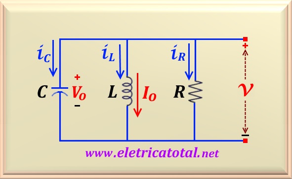
For this we consider a RLC circuit with all its elements connected in parallel, as illustrated in the Figure 24-01.
Figure 24-01
To analyze the circuit let's assume that both the capacitor and the inductor can have a stored initial energy,
either an inductor current or a capacitor voltage, both with nonzero initial values. In the circuit above these
initial conditions are represented as follows:
i (0+) = Ioandv(0+) = Vo
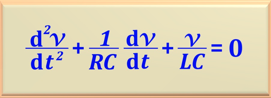
Applying the concepts of differential equation to the circuit we ccan get a second order linear homogeneous differential equation. Observe the equation below:
eq. 24-01
From the above equation we can determine the so-called characteristic equation of the equation
differential as shown below.
r 2 + (1 / RC) r + 1 / LC = 0
Since the differential equation is of second order, so we have a characteristic equation of second degree.
The solution obtained for v(t) depends on the roots of this second degree equation. So the two
roots are:
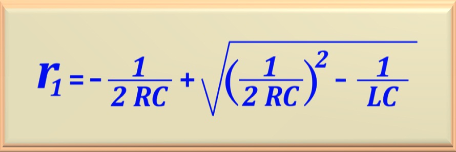
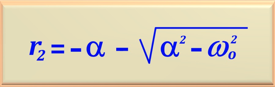
eq. 24-02
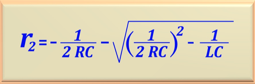
eq. 24-03
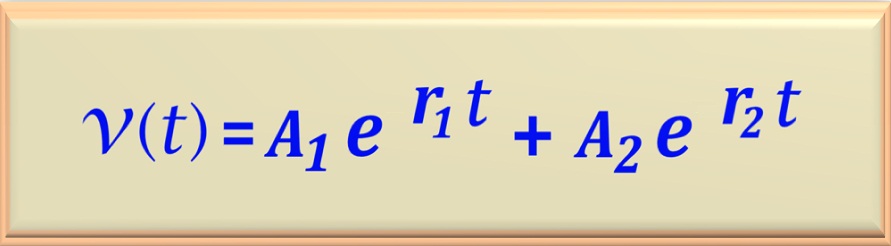
Now that we have the root values of the equation, we can write the solution of the differential equation. This is given by:
eq. 24-04
Note that the roots of the characteristic equation (r1 and r2) are determined by the
circuit parameters, R, L e C. The values of the constants A1 and A2
are determined by the initial conditions of the problem. Thus we can say that the general solution of eq. 24-01 has the
kind of the eq. 24-04.
Therefore, to find the solution of the problem, we must find the roots of the characteristic equation as the first step,
since the behavior of v(t) depends on the values of these roots. Note that the first part is the circuit response
due to the first root, r1. The second part is the circuit response due to the second root, r2.
We can call them solutions v1 and v2, respectively.
If v1 and v2 they are solutions, so we know that their
sum is also a solution. That is what the
eq. 24-04 are saying to us.
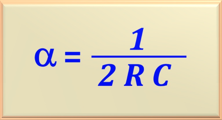
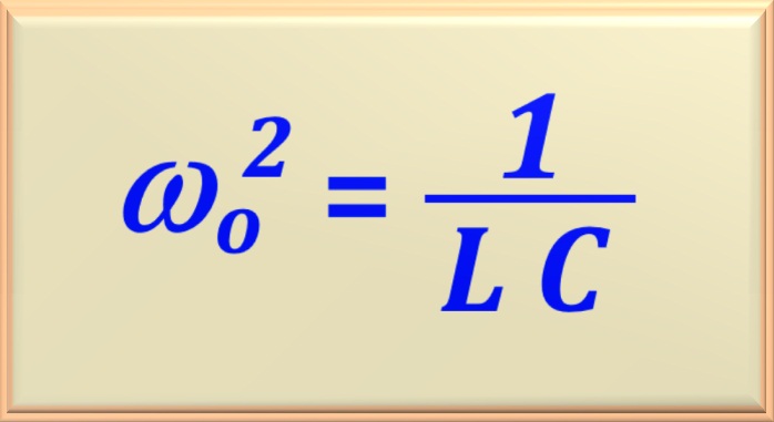
In practice, two new parameters are defined to rewrite the equations of the two roots. The first parameter, called the
Neper frequency or coefficient or damping factor, is represented by the greek letter alfa, α.
The second parameter,
called the resonant angular frequency or undamped resonant frequency,
is represented by the greek letter ωo.
So we can write them as:
eq. 24-05
eq. 24-06
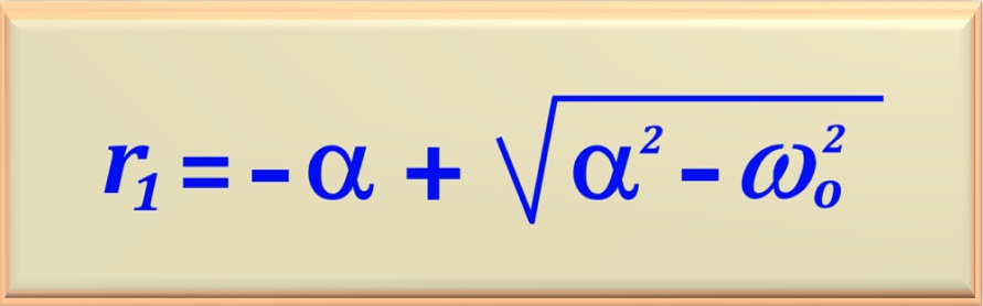
We are now able to write the root equations based on these two new parameters, or:
eq. 24-07
eq. 24-08
Making an analogy with what was studied in high school equations in high school, here we also realize that there are three
possible outcomes for radicating.
Positive - when α > ωo
Zero - when α = ωo
Negative - when α < ωo
These three possibilities give rise to three different types of circuit response. And each response type is given a
name that identifies it. So let's take a closer look at each case.
This answer happens when we have
α > ωo, and therefore the roots of the characteristic equation are
real, distinct and NEGATIVE. This condition implies that:
L C > (2 R C)2
For this case the answer is given by eq. 24-04 . The constants A1 and
A2 are determined by the initial conditions, more specifically by the values of
v(0+) and also by dv(0+) / dt, which are in turn determined by the initial capacitor voltage, Vo, and by the initial current of the inductor, Io.
We can summarize the procedure required to determine the response of an overdamped circuit..
1 - Find the roots of the characteristic equation, r1 and r2,
from the values of R, L and C.
2 - To determine v(0+) and dv(0+) / dt
using the circuit analysis methods previously studied.
3 - Calculate the values of A1 and A2 solving the system of equations consisting of the equations below.
v(0+) = A1 + A2
dv(0+) / dt =
iC (0+) / C =
r1 A1 + r2 A2
4 - Override the values of r1, r2,
A1 and A2 in the eq. 24-04 to get the expression of
v(t) to t ≥ 0.
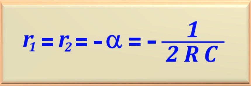
This answer happens when α = ωo, and therefore the roots of the equation
feature are real and EQUAL. This is the situation where the final state is reached as quickly as possible without oscillation in the system. In this case, the roots of the characteristic equation are:
eq. 24-09
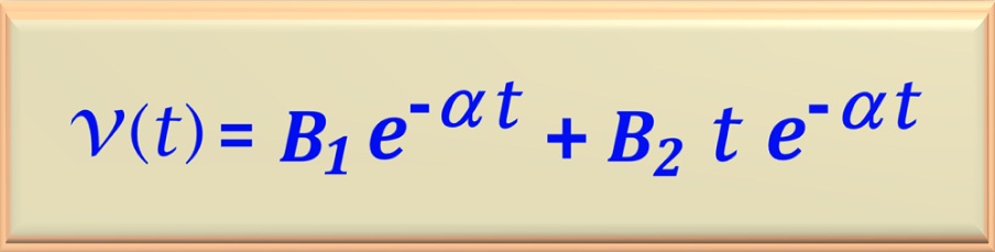
From what has been studied in the discipline differential equations, we know that when the roots of the characteristic equation are equal we cannot express the solution in terms of eq. 24-4. Then the solution must take the form of a sum of two terms: the first term is a simple exponential and the second term is the product of the independent variable by an exponential. Then the system response is given by the equation below.
eq. 24-10
To determine the values of B1 and B2, we use the same method as the previous item. Thus, we have the relations:
v(0+) = V0 = B1
dv(0+) / dt =
iC (0+) / C =
B2 - α B1
With the value of α given by eq. 24-09 and with the values of
B1 and B2, we can replace them in eq. 24-10 and find the equation solution of the circuit.
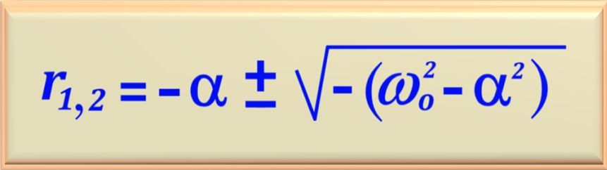
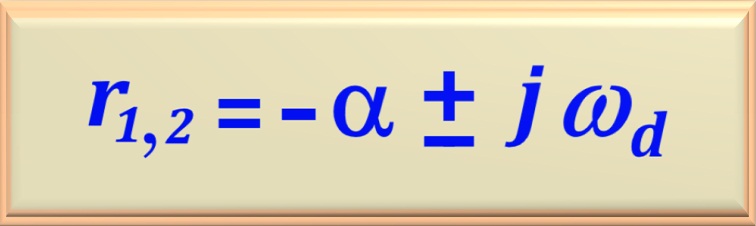
When α < ωo, the roots of the characteristic equation are
complex. So we say the circuit response is underdamped. Based on eq. 24-07 and
eq. 24-08, let's rewrite them more conveniently by making the following change:
eq. 24-11
Remembering that we can write j = √-1, so we can rewrite eq. 24-11 as:
eq. 24-12
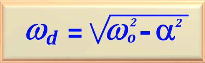
Note that we have redefined that is into of the root by a new parameter called damped angular frequency, ωd, conform the eq. 24-13.
eq. 24-13
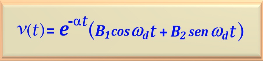
Thus, we can write the response of an underdamped parallel RLC circuit. The equation below is the result of some transformations and use of some properties of complex numbers.
eq. 24-14
The constants B1 and B2 They are real numbers. These coefficients are determined as we did for the other two cases. We calculate v(0+) and
your first derivative for t = 0+. In short we have
v(0+) = V0 = B1
dv(0+) / dt =
iC(0+) / C =
- α B1 + ωd B2
By eq. 24-14 we realize that the response is oscillatory due to trigonometric terms, that is,the voltage varies between positive and negative values. How often these oscillations occur depends on
of the value of ωd. On the other hand, due to the presence of the exponential function, the amplitude of oscillations decreases over time. How fast the amplitude of oscillations decreases
depends on α. For this reason the α parameter is called the
damping factor or damping coefficient. This also explains why the parameter
ωd is called damped angular frequency.
It should be noted that in the absence of damping, we have α = 0 and the frequency of the oscillations is ωo. In the presence of dissipative element, R in the circuit, α ≠ 0 and as a consequence,
ωd < ωo.
Then, when α is different from zero, we say that the oscillation frequency is
damped.
It is noteworthy that all calculations performed in the previous item, the circuit had no type of power source. Now let's study the behavior of the circuit when it contains power sources.
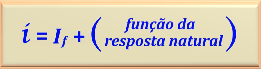
To obtain the response of a RLC circuit to a step function, we determine the voltage between the component terminals or the currents in the different branches. There may or may not be energy initially stored in the circuit.
The most direct way to solve the problem is to calculate the current in the inductive branch first. This current is of particular interest because it does not tend to zero for large values of t.
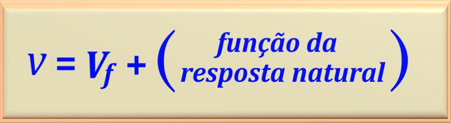
The solution of the second-order differential equation with a forcing function in the second member is equal to the sum of the natural response with the forced response. Thus, for the step function that has a constant value, the solution can be written as:
eq. 24-15
This is for the current case. In the case of voltage, the format is the same. So:
eq. 24-16
Where If and Vf represent the final value of the current and voltage in the response function.