In this chapter we will study resistors and inductors associations. We will see how the circuit behaves when subjected to an electrical voltage of the type Direct Current (DC).
A typical RL circuit is composed of a R resistor and a
L inductor in the serial configuration,
and are connected to a V voltage source via an electric switch S.
Initially we will consider that in the inductor no electric current circulates in its winding. Therefore, it has initial energy equal to zero. When this is not the case we will explain the initial condition.
The following are two fundamental properties of an inductor.
Based on the above properties the inductor assumes special characteristics when
subjected to variations in electrical current at its terminals. Usually a resistor is used
in series with the inductor to limit the electric current flowing through it. Like this,
when the inductor is abruptly subjected to a voltage variation
it behaves like an OPEN CIRCUIT, not circulating current through the inductor.
After this initial phase the current increases exponentially until reaching the
permanent regime. At this point the voltage on the
inductor is null, since there is no variation of electric current. So the inductor
behaves like a SHORT CIRCUIT.
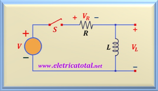
In the Figure 23-01 we can see a classic circuit to study the behavior of the inductor.
Figure 23-01
In this circuit we have a switch S that allows to turn on and off the voltage source that feeds the circuit. When closed it applies an electrical voltage from the voltage source V
to the circuit formed by the resistor in series with the inductor. In the technical literature
represents the key closing moment S by t = 0+.
The speed at which electric current flows in the inductor depends on the inductor inductance values and the electrical resistance of the resistor that is in series with the inductor.
The values of these two components determine the so-called time constant of the
circuit and is represented by the Greek letter τ (tau). Then we can write that:
τ = L / R
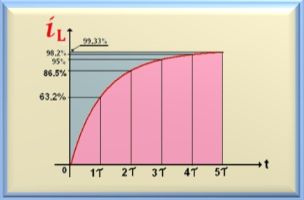
Figure 23-02
By applying abruptly an electrical voltage to the inductor, its inductance does not allow an instantaneous variation of the electrical current in the circuit to occur. Therefore, if there is no current flowing through the circuit then all the source voltage will be on the inductor. Like this, VL = V.
When the circuit begins to conduct electric current it rises rapidly
at the beginning and will reach the final value
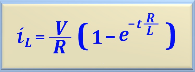
in an exponential way. See the Figure 23-02. This is what the equation below shows.
eq. 23-01
Note that as time grows the current in the circuit tends to the final value
iL = V/R.And about after five
time constants can say that the circuit has reached permanent regime.
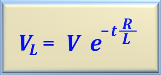
From that moment all the voltage of the source will be over the resistor and,
naturally, the voltage on the inductor will be zero. So to
calculations in electrical circuits we should consider the inductor as a
short circuit. This event can be described mathematically by equation below.
Note that when we studied the RC circuit it was evident that a capacitor after
electrically charged can maintain its electrical charge even if it is removed from the circuit.
The electric field established by the charge between capacitor plates is responsible for this. In an inductor this does not happen because the energy stored in an inductor
due to the magnetic field depends fundamentally on the current flowing through the inductor. If we remove the inductor from the circuit, current circulation ceases
and consequently the magnetic field ceases to exist. And this is why we realize
a spark when we turn off the power switch of an inductive circuit as
we produce a collapse of the magnetic field in the inductor and it reacts by dissipating its energy
in the form of a spark (high energy being dissipated in atmospheric air).
So let's look at how an inductive circuit behaves as shown below.
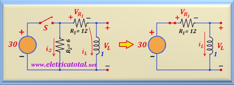
Figure 23-03
When we close the key S, the resistor R2 = 6 Ω is parallel to the
30 volt voltage source and the current flowing through it is independent of time. So to calculate
the current i2 just apply the Ohm's Law finding
i2 = 30/ 6 = 5 A. Since this current is constant to calculate
iL we can remove R2 from the circuit as it will not interfere with the calculations. So we get the circuit shown on the right side
from the Figure 23-03.
We know that by turning on the S switch, the inductor behaves like an open circuit.
Then for t = 0+, we concluded that iL = 0 , then VR1 = 0 and VL = 30 volts. After this moment the current
iL increases exponentially until reaching its value in steady state. We can calculate this value by Ohm's Law, because in steady state we know that the inductor behaves like a short circuit. So, iLfinal = 30/12 = 2.5 ampère. Attention should be paid to the fact that as the current iL increases, the voltage
VR1 also grows and consequently VL decreases until reaching
zero to times greater than five time constants.
We need to calculate the circuit time constant . But this is very easy,
because just apply the equation already seen, or:
τ = L / R1 = 1 / 12 = 0.08333 s = 83.33 ms
Thus using the equations studied in item 2 we can perfectly
calculate iL and VL, that is:
iL = 30/12 (1- e-(t/83.33 ) ms) = 2.50 (1- e- 12t) A
Note that for t = 0 we have iL = 0 and to t → ∞
we have iL = 2.50 A. For any other value of t, the current
iL will range from zero to 2.50 A.
And for the voltage on the inductor VL, we have:
VL = 30 e-(t/83.33 ) ms = 30 e- 12t volts
Do not forget that in the two equations above the time t is in seconds.
Similarly, in the case of VL, if t = 0 we have VL = 30 V and when t → ∞ we have VL = 0 V.
In this item, similar to what was shown for the RC circuit we have the equation that allows to relate the
electric current of an RL circuit to any moment. We will leave to show the use of this technique in the
solution of several problems presented in Problems
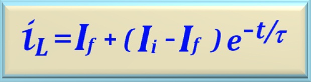
eq. 23-03
In this equation, the meaning of the variables are:
iL - current in the inductor at any time t
Ii - inductor initial current
If - final current in inductor
t - time we want to calculate the current iL
τ - circuit time constant
If you're interested in knowing how we got to this equation,
Click Here!
Just as we study the RC circuits, let's study the Thévenin Theorem
for RL circuits. So we have to find the Thévenin resistance of the circuit
which will be in series with the inductor. Thus we calculate the time constant of the
circuit. See the example below.
Example - Let's look at an example.
that appears on the page 351 (example 12.7) from the book of Robert Boylestad [3].
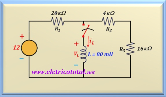
The circuit is shown in the Figure 23-04.
Item a - Let's determine the expression
mathematics for transient voltage behavior VL and of the current
iL as a function of time after key closure (at t = 0 s), knowing that the initial current in the inductor is zero.
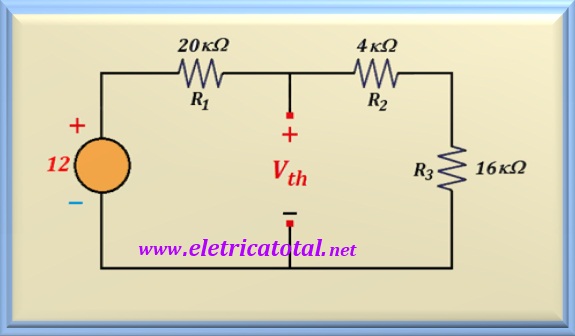
Figure 23-04
Considerations - Note that we have three resistors in the circuit
when the switch S is off.
To calculate the time constant , we must reduce to a single resistance, which will be the Thévenin resistance. To do so,
we know that we must short circuit the voltage source.
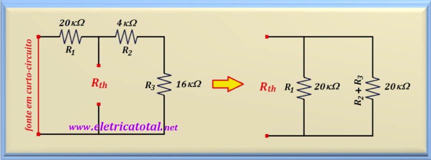
See in the Figure 23-05 how the modified circuit for the calculation of Thévenin resistance was.
Figure 23-05
Note that to the left of the figure above, the circuit with the voltage source appears.
shorted. We take the inductor from the circuit and we will calculate what the
resistance that the inductor "sees". This resistance is Thevenin's resistance,
Rth. Since we have two resistors of 20 kΩ each in parallel, so:
Rth = 10 kΩ
Now we must calculate Vth. As we know, the Thévenin voltage is
the open circuit voltage as shown in the Figure 23-06.
Figure 23-06
To calculate Vth just apply a resistive divider. Soon:
Vth = 12 x 20/ (20 + 20) = 6 V
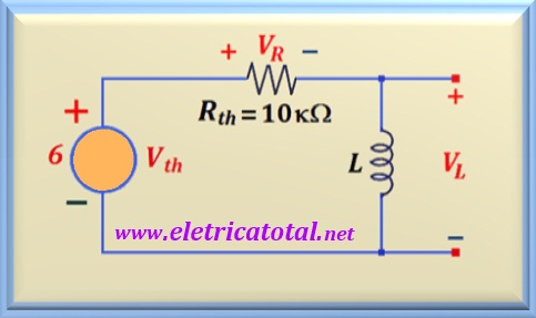
Knowing these values we can draw the Thévenin equivalent circuit,
as we can see in the Figure 23-07.
Figure 23-07
With this data we can calculate the values we need to
calculate the mathematical expression requested in the problem.
Let us calculate the time constant of the circuit, remembering that L = 80 mH.
τ = L / Rth = 80 x 10-3 H/ (10 x 103 Ω ) =
8 x 10⁻⁶ s = 8 µs
We can also calculate the maximum current that circulates through the inductor, taking into account consideration that for t > 5 τ we can assume the circuit on a permanent basis and,
in this case, the inductor behaves like a short circuit. Soon:
Imax = Vth / Rth = 6 V/ (10 x 103 Ω ) = 6 x 10⁻⁴ A
To find the mathematical expression that allows us to calculate the current iL, let's use eq. 23-1, already studied and shown below:
eq. 23-01
In this equation, V / R is the value calculated above using the value of
Vth / Rth, which is Imax. Soon:
iL = 6 x 10⁻⁴ (1 - e- t/(8 x 10-6) ) A
For the calculation of voltage, we will use eq. 23-2, or:
eq. 23-02
Where V is the value of Vth = 6 V, already calculated. Soon:
VL = 6 ( e- t/(8 x 10-6) ) volts
Thus we can calculate the mathematical expressions that define the behavior of the circuit at any time we wish.
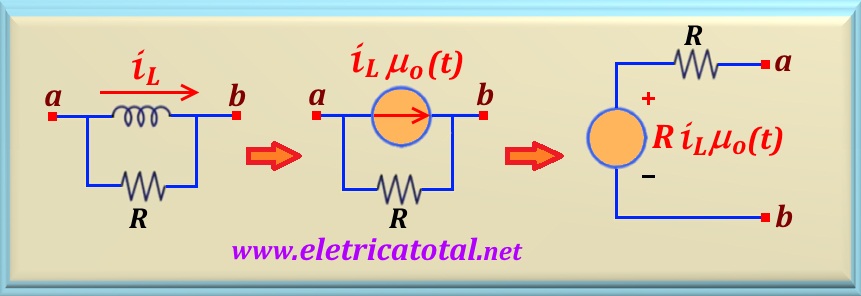
Many problems present, at a first instant (say in t = 0 - ), the necessary conditions to calculate the current in an inductor.
In a second instant, for example in t = 0+, we should use this information to find the solution of the problem.
In this case it is advantageous to replace the inductor with an
impulsive current source whose value will be the current in the inductor at time
t = 0-. See the Figure 23-08 for the transformations we can make that will help you find a solution
to the problem. To see an example
click here
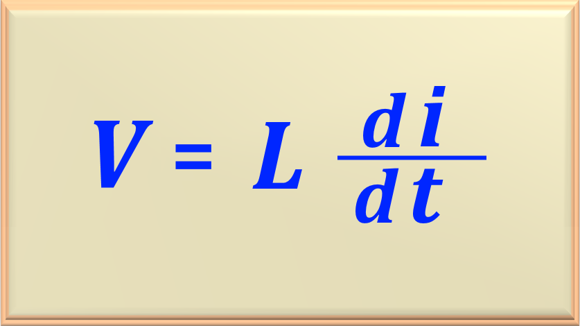
"The voltage at the terminals of an inductor is proportional to the temporal variation of the current in the inductor."
eq. 23-04
Note that the equation eq. 23-04 perfectly expresses the above definition. Therefore, two conclusions can be drawn:
If the current i through the inductor is constant, then the voltage across the inductor is zero, or V = 0.
If the current i in the inductor changes instantaneously, then V = ∞. Physically, this is impossible.
Example
To better understand this theory, let's analyze an example as shown below.
Be an inductor of 500 mH = 0.5 H fed by a current source given by the following function:
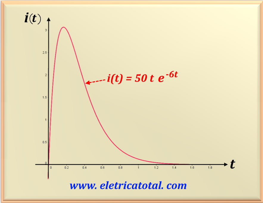
i (t) = 50 t e- 6 t u-1 (t) A
Note that when using the step function (u-1 (t) ) it means that the value of i(t) is only valid for t > 0. Considering t <0, the value of i(t)
is null. Let's create a graph, using Geogebra, showing the waveform of the current applied to the inductor. See the graph in Figure 23-09.
Figura 23-09
Note that from the graph in Figure 23-09 the function i(t) presents a maximum. We can determine when the maximum of the function occurs. To do this, we will differentiate the function i(t) and equate its value to zero. Thus, we can calculate at what time the maximum of the function occurs. We must pay attention that the function i(t) is the product of two functions.
So, to find the derivative of this function we must use the chain rule, that is, (u.v)' = v . u' + u . v'. Then i' (t) is:
i' (t) = 50 e- 6 t - 300 t e- 6 t = 0
eq. 23-05
50 e- 6 t = 300 t e- 6 t
Carrying out the calculation we find where the maximum of the function occurs.
t = 1/6 s
Entering this value into the function i(t) we will determine the maximum value that the current source provides to the inductor.
Carrying out the calculation, we have:
imax = 3,066 A
It is also possible to calculate the voltage across the inductor using eq. 23-04 and eq. 23-05. This way, we have:
vL (t) = 0,5 ( 50 e- 6 t - 300 t e- 6 t )
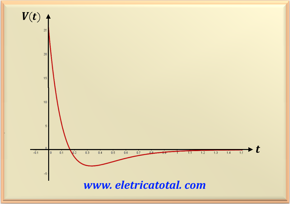
vL (t) = 25 e- 6 t ( 1 - 6 t )
Thus, we calculate the voltage across the inductor. See the graph of the function V(t) in Figure 23-10.
Figura 23-10
From these calculations it is possible to reach some conclusions. For example, using the function V(t) and the graph we see that the maximum voltage on the inductor (VL = 25 V )
occurs at t = 0. Therefore, we realize that the maximum current and the maximum voltage do not occur at the same instant, given that the voltage depends on the derivative of the current. Furthermore we see that
the voltage reaches the null value at the instant:
1 - 6 t = 0 ⇒ t = 1/6 s
Note that the voltage across the inductor was canceled when the current was maximum (t = 1/6 s as calculated previously), as this occurs when i' (t) = 0. After this moment, the voltage across the inductor reverses polarity, reaching a minimum value. Then it grows again until it disappears. To find when the voltage is minimum, simply differentiate the voltage function and set it equal to zero.
So, we will obtain:
v'L (t) = - 6 e- 6 t - 6 e- 6 t + 36 t e- 6 t = 0
Solving the above equation, we obtain:
t = 1/3 s
Substituting this value into the voltage equation we find the voltage value in the inductor at that moment, that is:
In many situations it is interesting to express the current in the inductor as a function of the voltage.
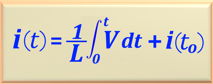
To do this, we can algebraically manipulate eq. 23-04 and arrive at:
V dt = L di ⇒ di = (V/L) dt
Applying the integral function to both members, we obtain:
eq. 23-06
Where i(t) is the current at time t and i(to) is the current at time to. Most of the time we have to = 0.
Note that i(to) has its own algebraic sign. If the direction of the initial current is the same as the reference direction of i, then it will be a quantity
positive. otherwise, i.e., the initial current is in the opposite direction, it will be a negative quantity.
Example
To better understand this theory, let's analyze an example as shown below.
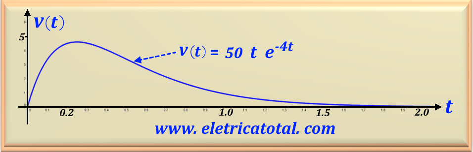
Let an inductor of 400 mH = 0.4 H be fed by a voltage source given by the following function:
v (t) = 50 t e- 4 t u-1 (t) V
Note that when we use the step function (u-1 (t) ) it means that the value of v(t) is only valid for t > 0. Considering t <0, the value of v(t)
is null. Let's create a graph, using Geogebra, showing the waveform of the voltage applied to the inductor. See the graph in Figure 23-11.
Figura 23-11
In the same way as was done in the previous example, we can determine the maximum of the voltage source by
deriving the function v(t) and setting its value equal to zero. Soon:
v' (t) = 50 (- 4 t e- 4 t + e- 4 t ) = 0
Solving this equation, we find:
t = 0.25 s
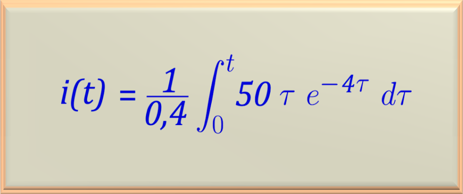
And to determine the current in the inductor we must use eq. 23-06. As we know, when we apply a sudden voltage variation to an inductor it behaves like a
open circuit and, therefore, the initial current in the inductor is null. Therefore, i(to) = 0. Then we have the following integral to solve:
To calculate this integral we must use integration by parts, as we have the product of two functions. So, applying this technique, we find: