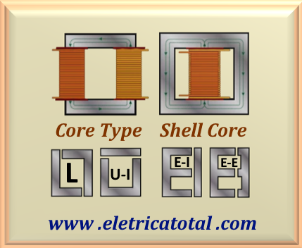
A single-phase transformer consists of a core composed of juxtaposed silicon steel sheets. In general,
these sheets are cut into some typical shapes, such as E and I or E and E.
Normally, this type of cut is used to form shell core. The cuts, type U and I or L,
are used to form core type. Note that all of them generate a closed path for the magnetic flux, as we can see in Figure 93-01.
Figura 93-01
Generally, materials are either hard or soft.
Hard materials are those in which magnetization tends to be permanent,
while soft materials are used in magnetic circuits of electrical machines
and transformers. They are related, although their uses are largely distinct.
Therefore, by adding coils made of copper or aluminum wires to these metal structures,
it is possible to build a transformer.
In the following items, we will address several characteristics of the transformer.
It is worth noting that, in the study of magnetism, certain variables can be expressed in several units. In some books, some units linked
to the old CGS system are still mentioned. Let's look at some relationships.
In the International System, SI, the unit of measurement for magnetic flux is the weber
and that for magnetic induction density,B or also known as magnetic flux density, is measured in
Tesla, and is equivalent to 1 Wb / m2. However, texts and books are still produced where the
magnetic flux density is expressed in gauss, G, a unit of the CGS system. The correspondence
between T and G is 1 T = 10,000 gauss. On the other hand, the
magnetic field intensity,H, has the dimension of ampere-turns per meter in the SI
system. And in the CGS system, its unit is the oersteds, Oe. So, one oersted means that this magnetic
field intensity is needed to generate a magnetic flux density of one gauss in free space.
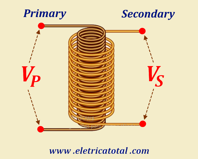
Why do transformers use silicon steel cores? To answer this question, let us take as a reference two coils very close to each other,
as shown in Figure 93-01.1, noting that there is no physical contact between them, as they are completely isolated and
immersed in air (magnetic medium).
Figura 93-01.1
Let's designate the primary inductance as L1 and the secondary inductance as L2.
Between these two windings there is a coupling determined by the mutual inductance, M
( See Here !!).
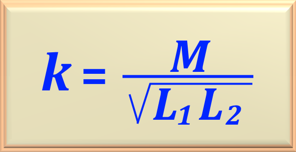
Thus, these variables are related by the coupling coefficient, according to eq. 78-07 below.
eq. 78-07
Analyzing this equation, we conclude that, if L1 = L2 = L = M, the result is k = 1,
something physically impossible. Therefore, the objective is to maximize the value of M.
Two equations already studied will be recalled below.
H = B / μoandH Ln = N I
We are considering that the magnetic medium is air. By joining these two pieces of information, we obtain the following equation.
B = μo N I / Ln
As we know, the value of μo is very small. Its value is
μo = 4 π x 10-7 H/m.
Considering, in this equation, μo and Ln as constants,
the variables that we can vary are I and N.
Therefore, to obtain a value of B that can be used in transformers,
high values of I and N would be necessary. This, in itself, makes the use of materials with low magnetic permeability unfeasible.
Conclusão
"We conclude that in electrical machines (transformers) it is necessary to use materials with high magnetic permeability,
such as silicon steel."
The silicon steel sheets that make up the core of transformers and electrical machines in general have exceptional magnetic properties.
They are composed of an iron alloy with the addition of silicon, generally varying between 2% and 4.5% of their composition.
As they have a very narrow hysteresis curve, this means that hysteresis losses are reduced, resulting in lower energy
losses during magnetization and demagnetization cycles. In addition, their high magnetic permeability facilitates
the induction of strong magnetic fields with reduced magnetization currents, further reducing losses.
On the other hand, despite being a ferromagnetic material, silicon steel has low electrical conductivity, which minimizes eddy
currents that form in the core. These eddy currents also contribute to energy losses in the transformer.
Due to all these properties, the use of silicon steel in electrical machines makes it possible to build highly efficient devices.
With the aim of further improving the properties of silicon steel, the silicon steel industry is undergoing constant technological advances.
Currently, there are three types of silicon steel:
Grain-oriented silicon steel - They have a crystal structure aligned in such a way as to optimize magnetic properties.
These steels present even lower hysteresis losses, allowing the construction of even more efficient machines.
Non-grain-oriented silicon steel - In addition to grain-oriented steels, there are also non-grain-oriented
silicon steels, which have more isotropic magnetic properties. These materials are particularly useful in applications where the
direction of magnetic flux is not constant, such as in electric motors.
Refined grain silicon steel - Another important innovation is the development of silicon steels with refined grains,
that is, with a smaller crystalline structure. This characteristic results in lower eddy current losses,
further improving the efficiency of electrical devices.
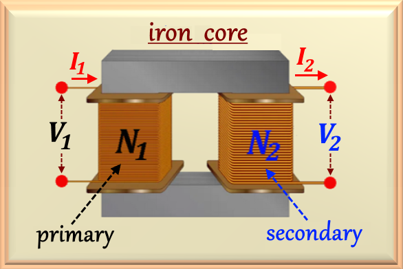
We can define a transformer as a static machine that transforms AC electrical power at a given voltage and
current level to another voltage and current level, using a magnetic field as an intermediate medium.
Basically, it is formed by two or more windings, electrically isolated from each other, having a certain electrical resistance
and self-inductance. These windings are coupled via a mutual inductance (M), that is, they are mutual magnetic
fluxes that must be obligatory variable over time for the phenomenon of self-induction to exist, which, in turn,
will produce the electromotive force (EMF) in the windings. mutual inductance was studied in more
detail in Chapter 78.
The reader can access ☞Clicking Here !!
The reason for this phenomenon is basically due to the non-linearity of the hysteresis present in all magnetic materials.
Figura 93-02
Suppose the transformer shown in Figure 93-02 is supplied with a sinusoidal voltage V1.
Considering the internal voltage drop in the transformer being much smaller than the applied voltage V1, the induced EMF
must also be sinusoidal and thus, the flux established in the core must also be. Therefore, a current flows in the
primary circuit, even when the
secondary circuit is open circuit. This current is necessary to establish the
flux in a real ferromagnetic core, as explained in Chapter 92. It consists of two components:
1 - The magnetizing current Ip, the current required to produce the flux
in the transformer core.
2 - The core loss currents Ih and Im are the currents responsible
for the hysteresis and eddy current losses in the core.
For a better understanding, let's reproduce the electrical diagram of a real transformer model, as studied in Chapter 92. See Figure 93-03.
Figura 93-03
Note the model above. E1 represents the so-called counter electromotive force,
the voltage that opposes the voltage applied to the primary, V1. If V1
is constant, then E1 will also be constant, as will the magnetic flux in the transformer core.
This constancy of values must be maintained regardless of the electric current supplied by the secondary to the load.
Therefore, the primary winding must absorb from the feeder line, in addition to the magnetizing current, an electric
current I'1. This current is called the
primary reaction current.
Furthermore, the flux must lag behind the induced EMF by 90°. A transformer requires less magnetic material
if it operates at a higher magnetic flux density. Therefore, from an economic point of view, a transformer is designed to operate close
to the saturation region of the magnetic core, although this increases the presence of harmonics in the wave.
When the voltage applied to the primary of a transformer is sinusoidal, the mutual flux established in the core is considered
sinusoidal. The no-load current, IP (exciting current), will be non-sinusoidal due to the hysteresis loop
containing the fundamental harmonic and all odd harmonics.
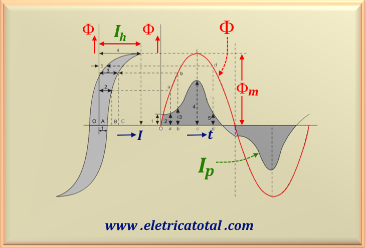
Consider the core hysteresis loop as shown in Figure 93-04.
We know that Φ = B A and I = (H Ln ) /N. Thus,
the hysteresis loop is plotted in terms of flux Φ and current I rather than B and H,
so that the current required
to produce a given value of flux can be read directly. The no-load current waveform, IP,
can be found from the sinusoidal flux waveform and the Φ - I (hysteresis loop) characteristics of the
magnetic core. The graphical procedure for determining the IP waveform is shown in Figure 93-04.
Figura 93-04
We observe that the no-load current waveform presents odd harmonics, such as the third, fifth and other higher orders,
which rapidly intensify as the maximum flux approaches saturation. However, the third harmonic is the most relevant.
For most applications, harmonics above the third order can be considered insignificant. In the no-load current, the
contribution of the third harmonic corresponds approximately 5% to 10% of the fundamental at nominal voltage.
In load situations, the total primary current corresponds to the phasor sum of the load current and the no-load current.
Because the magnitude of the load current is significantly greater than that of the no-load current, the primary current
appears almost like a sinusoidal wave in practical terms during operation under load. Therefore,
when the transformer operates in the saturation region, the magnetizing current has a higher proportion (30 to 40%) of harmonics.
"When a transformer is operated in the saturated magnetizing region, the magnetizing current waveform is even more
distorted and contains a higher percentage of harmonics."
Therefore, for economic reasons, transformers are usually designed to operate in the saturation region.
When a transformer is designed for this region, it requires a smaller amount of magnetic material.
For the moment, ignoring the effects of the stray flux, we see that the
mean flux in the core is given by
Φmed = (1/ NP) ∫ V1 (t) dt
So if the primary voltage is written as V1(t ) = Vmax cos (ωt ) V, the resulting average flux will be
Φmed = (Vmax / ω NP) sen (ωt )
eq. 93-01
Where the variables are:
Φmed - average flux in the transformer's magnetic core;
NP - number of turns in the transformer's primary winding;
Vmax - maximum voltage of the sinusoid, or √2 Vrms;
ω - angular velocity of the sinusoid, or ω = 2 π f.
If the values of the current required to generate a given flux are compared with the flux in the core, for various values,
we can construct a simple graph of the magnetizing current flowing in the core winding. This graph is shown in the lower part of Figure 93-04.
With respect to the magnetizing current, we should note the following points:
1 - The magnetizing current in a transformer is not sinusoidal. The higher frequency components of the
magnetizing current are due to the magnetic saturation of the transformer core.
2 - When the peak flux reaches the core saturation point, a small increase in this peak
requires a large increase in the magnetizing current.
3 - The fundamental component of the magnetizing current lags the applied voltage by 90°.
4 - The higher frequency components of the magnetizing current can be quite large when compared
with the fundamental component. In general, the more a transformer is saturated, the larger its harmonic components will become.
When operating the transformer without load, or at no load, it is necessary to supply a current to supply the power required
by hysteresis losses and losses due to eddy currents in the core. This current is called the loss current in the transformer's
magnetic core. Assume that the magnetic flux in the core is sinusoidal. Since the eddy currents in the core are proportional
to the derivative of the magnetic flux with respect to time (dΦ/dt), they reach their maximum value
when the flux in the core passes through zero Weber. Therefore, the loss current in the core reaches its maximum
value when the magnetic flux passes through zero.
Regarding the loss current in the transformer's magnetic core, it is important to note that:
1 - Due to the non-linear effects of hysteresis, the currents involved in core losses also do not follow a linear behavior.
2 - The fundamental component of the core loss current is in phase with the voltage applied to the core.
The total current in the no-load core is called the exciting current of the
transformer. It is simply the sum of the magnetizing current and the
core loss current.
In a well-designed power transformer, the exciting current is much smaller than the
full-load current of the transformer.
The magnetizing current of a transformer is in the order of 3 to 5% of the nominal current. This occurs
when the transformer is operating in the steady state. However, when the transformer is energized
for the first time, there may be a sudden transient current circulation in the primary winding, with a high magnitude.
The flux may reach a maximum value equivalent to twice the usual flux. This causes the core to saturate,
resulting in a high peak in the magnetizing current.
This current, called inrush current, can reach values between 10 to 20 times the value
of the nominal current of the transformer.
The value of the inrush current depends on the instant at which the transformer is connected to the power supply network.
The inrush current will be maximum when the input voltage passes through the value zero. This current is minimized
when the input voltage passes through its maximum value, that is, at the peak. However, in practice, it is
not possible to select a specific instant in time to activate the switch connecting the transformer to the power supply network.
Thus, high values of the inrush current generate mechanical forces of great magnitude on the transformer windings.
Therefore, the windings must be firmly fixed around the core to withstand great mechanical forces without moving,
which could seriously compromise the transformer's performance or even lead to its destruction.
When a transformer is connected to supply power, in the worst case scenario, the transient inrush current causes a
high value of magnetic flux in the core. The flux in the core can reach twice the normal value. This is called the
doubling effect of the magnetic flux.
It is important to consider that when a transformer is disconnected from the supply network, it may
not be possible to reduce the magnetic flux to zero. For this reason, the transformer core retains
some residual flux, which we will call Φr.
Let's assume that the secondary of the transformer is open circuit and that, in the primary, we apply a sinusoidal voltage, or:
v1 = Vmax sen ( ωt + φ )
eq. 93-02
In the equation above, Vm represents the maximum voltage applied to the transformer primary,
while φ represents the angle of the sinusoidal voltage, at the instant t = 0.
Assuming, for a moment, that the losses in the core and in the resistance of the primary winding are neglected, we can write that:
v1 = N1 ( dΦ / dt )
eq. 93-03
In the equation above, N1 is the number of turns of the primary winding and Φ is the flux
in the transformer core. Considering that the flux is given by:
Φ = Φm sen ( ωt )
Deriving the above equation and considering that the flux reaches its maximum value when cos ωt = 0, we can express for the
steady state, that:
Vmax = ω Φm N1
eq. 93-04
From eq. 93-02 and eq. 93-03, we have:
dΦ / dt = ( Vmax / N1 ) sen ( ωt + φ )
eq. 93-05
Substituting eq. 93-04 into eq. 93-05, we obtain:
dΦ / dt = ( ω Φm ) sen ( ωt + φ )
eq. 93-06
Now, integrating eq. 93-06, we obtain:
Φ = - Φm cos ( ωt + φ ) + Φc
eq. 93-07
Here, Φc represents an integration constant. Its value can be determined from the
initial conditions for t = 0. Consider that, when disconnected from the supply network, the transformer retained
a small residual magnetic flux, Φ = Φr, in its core. Thus,
for t = 0, we have Φ = Φr.
Substituting this value into eq. 93-07, we have:
Φr = - Φm cos ( φ ) + Φc
eq. 93-08
Φc = Φm cos ( φ ) + Φr
eq. 93-09
Using the value of Φc given by eq. 93-09 and substituting it into eq. 93-07,
we obtain an equation with two terms, as in eq. 93-10 below.
Φ = - Φm cos ( ωt + φ ) +
(Φm cos ( φ ) + Φr)
eq. 93-10
Note that the portion between the red parentheses represents the transient component, while the
other portion represents the steady state. And the magnitude of the transient component is given by
eq. 93-09 and is a function of φ, where φ is the instant at which the transformer is connected to the power grid.
So, if the transformer is connected at the instant φ = 0, we have cos φ = 1 and eq. 93-09,
becomes:
Φc = Φm + Φr
eq. 93-11
Under this condition, eq. 93-10 results in:
Φ = - Φm cos ( ωt ) +
Φm + Φr
eq. 93-12
Another condition we can study is when ωt = π. In this case, we have cos π = -1, obtaining:
Φ = 2 Φm + Φr
eq. 93-13
Thus, the maximum value of the magnetic flux in the core is greater than twice the nominal flux.
Consequently, the core suffers a high saturation. The magnetizing current required to produce such flux in the
core can be up to 10 times the value of the nominal primary current. Therefore, we can conclude that:
"This inrush current can produce electromagnetic forces about 25 times higher than the normal value.
Therefore, the windings of large transformers are strongly fixed to prevent displacement."
As previously stated, for there to be no inrush current, it is necessary that, when the transformer is connected to the power grid,
the supply voltage is at its positive or negative peak. We should add that other transformers in the system, load currents in the system,
capacitances distributed throughout the grid, all contribute to reducing the inrush current.
In the analysis of electrical transformers, we consider two types of losses: copper losses and core losses.
Core losses correspond to magnetic losses, which occur due to hysteresis and eddy currents.
We will study the two separately.
When a coil is surrounded by a changing magnetic flux, it induces an EMF in the coil according to Faraday's law.
If this coil is wrapped around a magnetic material, an EMF will also be induced in the magnetic material by the same
magnetic flux. Since the magnetic material is also a good electrical conductor, the EMF induced within the material
causes electric currents to appear within it, called eddy currents or eddy currents. The location and path of this current
causes it to surround the magnetic flux that produces it. In fact, there are as many closed paths around the magnetic
field within the magnetic material as one can imagine.
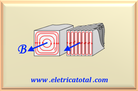
On the left side of Figure 93-05, we can see
some of the paths for the currents induced in a solid magnetic material when
the flux density is increasing with time.
As the flux in the magnetic material increases, so does the
induced EMF in each circular path. The increase in the induced EMF results in an increase in the
eddy current in that path. As a result of this current, energy is converted
to heat in the resistance of the path. By adding together the power loss in each closed loop
within the magnetic material, we obtain the total power loss in the magnetic
material caused by the eddy currents. This power loss is called the
eddy current loss.
Eddy currents establish their own magnetic flux, which tends to oppose the original magnetic flux. Therefore, eddy
currents not only result in eddy current losses within the magnetic material, but also exert a demagnetizing effect on the core.
Consequently, a larger MMF is required to produce the same magnetic flux in the core. Demagnetization intensifies as
we approach the core axis. The overall effect of demagnetization is to bunch up the magnetic flux toward the outer surface of
the magnetic material. This makes the inner part of the core magnetically ineffective.
Figura 93-05
Due to all these factors, it is necessary to adopt measures that minimize these effects. One way to minimize the adverse
effects of eddy currents is to make the magnetic core highly resistive in the direction in which eddy currents tend to flow.
We can do this in practice by stacking thin pieces of magnetic materials to form a magnetic core, as shown on the right side
of Figure 93-05. The thin piece, known as a lamination, is coated with varnish or shellac and is commercially available
in thicknesses ranging from 0.36 mm to 0.70 mm. The thin coating thus makes each lamination reasonably
well electrically insulated from the others. In addition, the magnetic core constructed of these laminations forces eddy currents
to travel long, narrow paths within each lamination. The resulting effect is to reduce eddy currents in the magnetic material.
In free space (nonmagnetic material), the permeability μo is constant. Thus, the relation B - H is linear.
However, in the case of ferromagnetic materials used in electrical machines, this is not the case, where the relation B - H is strictly
nonlinear in two respects: saturation and hysteresis.
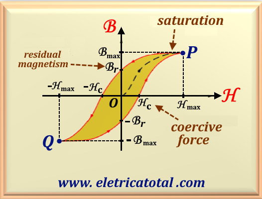
The hysteresis nonlinearity is the double-valued B - H relation exhibited in the variation of the H cycle
as shown in Figure 93-06.
Figura 93-06
Starting at point O and a little beyond this point, the curve presents a non-linearity. In the middle of the curve,
it presents an "almost" linearity, ending with a region of saturation. In this region, the B field
increases much less quickly than H. Near the point P, the saturation is quite pronounced and the magnetic
material behaves like free space.
For economic reasons, electrical machines and transformers are designed to work a little beyond the beginning of the saturation zone.
Hysteresis in electrical machines gives rise to the so-called hysteresis loss. These losses are caused by the variation of the
magnetization cycle, that is, the material undergoes magnetization in one direction and, subsequently, the direction is reversed.
Thus, energy is lost due to molecular friction in the material, that is, the magnetic domains of the material resist being
rotated first in one direction and then in the other.
Therefore, the magnetic material requires extra energy to overcome this opposition. We can state that these losses per unit volume
of the magnetic material in each magnetization cycle are proportional to the area of the hysteresis cycle. We should also note that,
if the temperature of the machine increases, the hysteresis losses also increase.
The most commonly used ferromagnetic materials in transformers and electrical machines are cast iron,
cast steel and the best of them, silicon steel. Each of these materials presents a characteristic curve as shown in Figure 93-07.
Figura 93-07
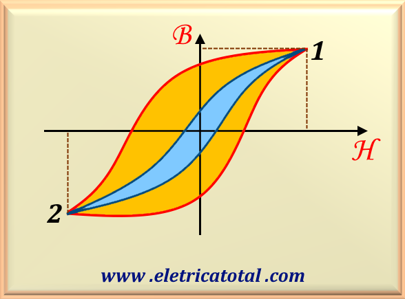
Regarding the use of the hysteresis loop, it should be noted that in transformer and electrical machine designs,
the chosen magnetic material is one that presents a very narrow hysteresis loop, as this means low losses.
In Figure 93-08, the hysteresis curve in blue satisfies this requirement. When the interest is to produce
permanent magnets, then the chosen magnetic material is one that has a very wide hysteresis loop,
as this material presents a high coercivity value. This case is shown in Figure 93-08 by the hysteresis curve in orange.
5.3 Separation of Hysteresis Losses fromParasitic Losses
When we connect the primary winding to the mains, the transformer core is subjected to magnetization at the mains frequency.
Therefore, a certain amount of energy is wasted in this process.
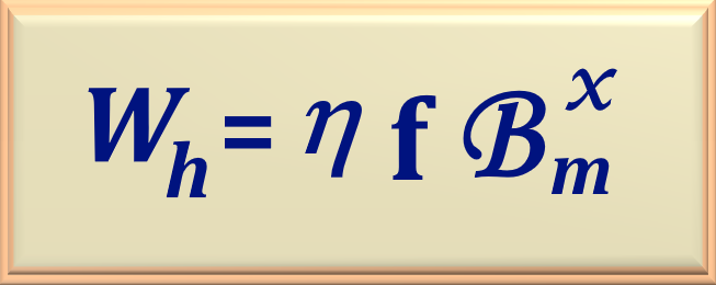
The hysteresis losses, Wh, as stated in the previous item, depend on the area of the hysteresis loop
and the material used in the core. These losses can be expressed by eq. 93-14.
eq. 93-14
In this equation, the variables involved are:
Wh - Hysteresis loss in W.
η - This is the Steinmetz constant and depends on the ferromagnetic material.
f - Power grid frequency in Hz.
Bm - Maximum magnetic flux density.
x - For steel, it can vary from 1.5 to 2.0.
It is important to consider that, when we add small percentages of silicon to the steel, the hysteresis loop becomes
smaller and, consequently, there is a reduction in hysteresis losses.
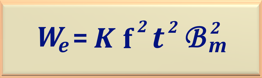
On the other hand, when variations in the magnetic flux occur, currents are induced in the ferromagnetic material,
causing parasitic losses (eddy loss). These losses are directly proportional to the squared
of the thickness, t, of the laminations used in the manufacture of the transformer core.
The parasitic losses, We, can be written as eq. 93-15.
eq. 93-15
In this equation, the variables involved are:
We - Eddy current loss in W.
K - It is a constant.
f - Frequency of the electrical network in Hz.
Bm - Maximum magnetic flux density.
t - Thickness of the sheet used in the manufacture of the core.
Thus, the sum of the parasitic losses and the hysteresis loss results in the total iron losses, Pfe, given by eq.93-16.
eq. 93-16
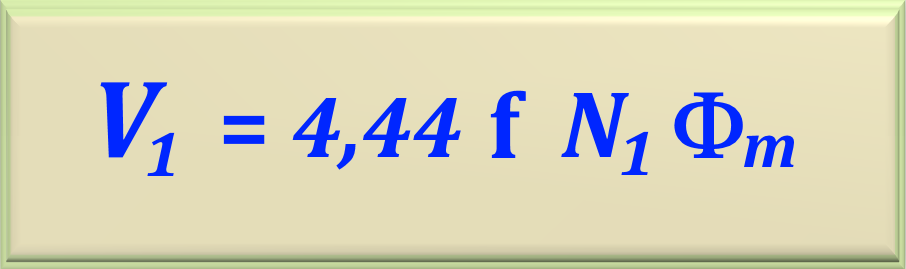
Remembering what was studied in chapter 91, the electromotive force (EMF) induced in the windings of a transformer
is given by eq. 91-12 or eq. 91-13. For better understanding, let's repeat eq. 91-12 below. This equation
represents the effective or RMS value of the induced voltage. The reader can access this item ☞Magnetic Flux and Induced Voltage
eq. 91-12
Recalling eq. 75-11a where Φm = A Bm
and substituting this value into eq. 91-12, we obtain:
E = V = 4.44 A Bmf N
In the equation above, setting K = 4.44 A N, we can rewrite it as follows:
E = V = K Bmf
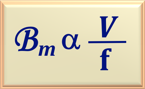
Analyzing the equation above, we can easily conclude that the value of Bm
is proportional to the ratio V / f.
Mathematically, we can write:
eq. 93-17
Therefore, this equation indicates that Bm will remain constant as long as the ratio
between the applied voltage and the
frequency of the power grid is also kept constant.
Using eq. 93-04 and those developed earlier, we can write:
Pfe = η fBmx + K f2 t2Bm2
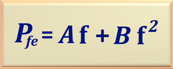
Thus, keeping the ratio V / f constant, we obtain Bm constant. Then, it is possible to write
the following relation:
eq. 93-18
In this equation, A and B are constants to be determined. Thus, it is possible to determine the values of these constants by measuring the
total losses in the iron,
Pfe, at two different frequencies, keeping the ratio V / f constant. In this way, we obtain
a system of two equations with two unknowns, whose solution is simple, as will be demonstrated below.
Pfe1 = A f1 + B f12
Pfe2 = A f2 + B f22
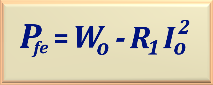
By performing a no-load test on the transformer, we can determine the value of the iron losses, Pfe, by
reading the value measured by the wattmeter, W, and subtracting the loss caused by the resistance of the primary winding.
Mathematically, we can write:
eq. 93-19
Therefore, we must perform a no-load test on the transformer at two different frequencies, f1 and
f2.
In both situations, it is necessary to adjust the voltage V to keep the value of Bm constant. Thus, it is possible to separate
the two components of the losses: loss due to hysteresis and
loss due to eddy currents.
To better understand the application of this technique, access the problems
Problem 93-9 and
Problem 93-10
This item was studied in the previous chapter (Real Transformer). Let us repeat it here.
The presence of the iron core causes a loss because energy is needed to magnetize the core.
To represent this loss in the electrical model of the transformer, we add inductance in parallel with the
primary winding, symbolized in the model by a reactance designated as Xm.
In addition, we must provide a resistance in parallel with this reactance to represent the losses that occur
due to the presence of hysteresis and eddy currents that exist in the iron core. This resistance
is symbolized by Rh in the electrical model of the transformer,
as can be seen in Figure 93-09.
Note that in the circuit model we have the voltage E1 across the magnetizing circuit. The current
Ih across the resistance Rh is in phase with E1. However,
the current Im, which flows through Xm, lags behind 90° in relation to
E1. Thus, we can relate the three currents, that is, Ip,
Ih and Im through the equation eq. 93-20 below.
eq. 93-20
Figura 93-09
Note in the model above, E1 represents the so-called counter electromotive force,
a voltage that opposes the voltage applied to the primary, V1. If V1 is constant,
then E1 will also be constant, as will the magnetic flux in the transformer core. This constancy of
values must be maintained for any electric current that the transformer secondary supplies to the load. Thus, the primary
winding must absorb from the feeder line, in addition to the magnetizing current, an electric current I'1.
This current is called the primary reaction current.
The total magnetic flux linked with the primary winding can be divided into two components: the resulting mutual flux,
which is confined to the iron core and is the result of the combined effect of the electric currents in the primary and secondary;
and the stray flux of the primary and secondary, which is linked with itself. On the other hand, most of the stray flux is
in the air. Since air does not undergo saturation, the stray flux and the voltage induced by it vary linearly with the
primary current I1. This effect can be simulated, in the electrical model, by a stray reactance
represented by Xm, as shown in Figure 93-09.
We must not forget that copper or aluminum wires are used to make transformer windings, and therefore they present
electrical resistance. These resistances cause losses due to the Joule effect and are represented in the electrical model by R1
(primary) and R2 (secondary).
Therefore, it should be clear that the voltage V1 opposes
three phasor voltages: the voltage drop across the primary resistance R1,
the voltage drop across the stray reactance X1, and the back electromotive force E1
induced in the primary by the resulting mutual flux.
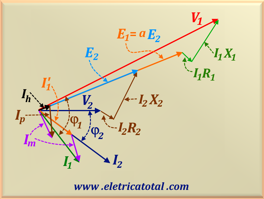
Based on the circuit shown in Figure 93-09, it is possible to develop a phasor plot of the transformer.
See Figure 93-10 for the plot with all the details presented by the circuit.
Figura 93-10
Resume
In short, in order to study the model of a real transformer we must consider four essential points.
1 -Copper Losses: (R I2) due to the heating of the wires by the
passage of the electric current. They are proportional to the square of the electric current.
2 -Losses by Eddy Currents: due to the heating of the transformer core caused by the
magnetization of it and are proportional to the square of the voltage applied to the transformer.
3 -Hysteresis Losses: due to the change in the configuration of the transformer core
magnetic domains and is a nonlinear function of the voltage applied to the transformer.
4 -Leakage Flux: is the flux that does not include the primary and secondary
transformer windings and their losses are represented by the leakage inductance of each winding.
Attention
"It is noteworthy that in a good transformer design, the power dissipated in
the primary winding resistance must be equal to the power dissipated in the
secondary winding resistance."
Thus, by performing two tests (studied below) on the transformer, we were able to determine the value of
resistances of the primary and secondary.
As for reactances , it follows the same principle and with the two tests mentioned above we can determine their values as well as the values of Rh and Xm.
There is another approach to solving transformer circuits that eliminates the need for explicit voltage level
conversions at each transformer in the system. Instead, the necessary conversions are performed automatically
by the method itself, without the user having to worry about impedance transformations. Since these impedance
transformations can be avoided, circuits containing many transformers can be solved easily with less possibility of error.
This method of calculation is known as the per unit (pu) system of measurement.
Thus, when an electrical machine is designed or analyzed using the actual values of its parameters, it is not immediately
obvious how its performance compares with that of another machine of a similar type. However, if we express the parameters
of a machine as a per-unit (pu) of a base (or reference) value, we find that the per-unit values of machines of the same
type but with widely different ratings fall within a narrow range. This is one of the main advantages of a per-unit system.
An electrical system has four quantities of interest: voltage, current, apparent power, and impedance. If we select base values
of any two of these, the base values of the remaining two can be calculated.
To implement this system, it is necessary that each electrical quantity be measured as a decimal fraction of some level
that serves as a base. In the per unit, pu system, we must choose two quantities as the base values. Usually, the ones
chosen are voltage and power (or apparent power). Once these base quantities have been chosen, all other base quantities are
determined from them, according to the fundamental electrical laws.
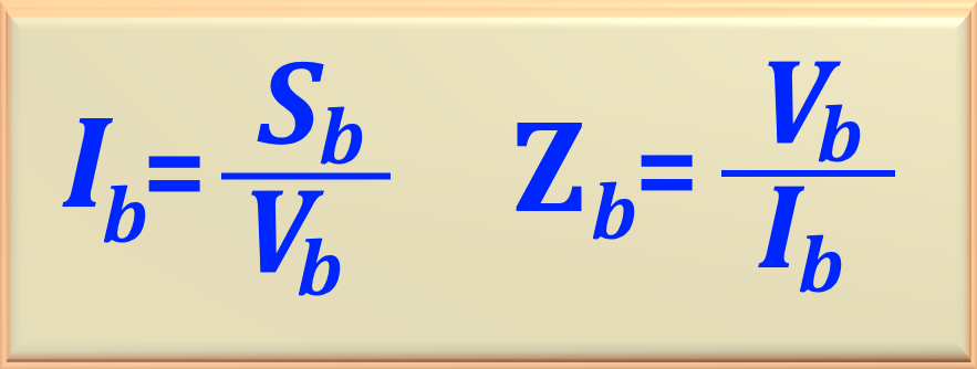
Thus, if Sb is the base of apparent power and Vb is the base of electrical voltage,
then the base of electrical current and impedance are:
eq. 93-21
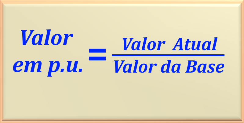
Thus, the value in pu of the desired quantity can be written as a decimal fraction of the value of base, according to eq. 93-22 below.
eq. 93-22
Therefore, it is convenient to compare quantities in their p.u. values corresponding to full load conditions.
For a better understanding of this technique, let's look at an example.
Example 93-01
Let's assume a 50 kVA, 10,000/220 V transformer. The primary impedance is 44 + j220 Ω.
Find the primary impedance in p.u..
Solution
Let's take the magnitudes electrical voltage and apparent power as a basis. Therefore:
Vb = 10.000 V and Sb = 50.000 VA
Now, we can calculate the base imedance of the primary circuit.
Zb = Vb2 / Sb = 10.0002 / 50.000
Performing the calculation, we obtain:
Zb = 2.000 Ω
Thus, the primary impedance at p.u. is:
Z1, pu = 44 + j220 Ω / 2.000 Ω = 0,022 + j 0,11 pu
Um transformador pode ter múltiplos enrolamentos que podem ser conectados em série
para aumentar a tensão nominal ou em paralelo para aumentar a corrente nominal. Antes
das conexões serem realizadas, no entanto, é necessário que saibamos a polaridade de
cada enrolamento. Por polaridade, queremos dizer a direção relativa da força eletromotriz induzida (FEM) em
cada enrolamento.
A polaridade de um enrolamento refere-se à característica
que mostra a dependência do sentido da FEM induzida em
relação ao fluxo que a gera (normalmente assinalada com
uma seta ou um ponto). Assim, dois terminais de dois
enrolamentos são da mesma polaridade ou homólogos
quando estiverem igualmente situados relativamente ao
sentido positivo num e noutro enrolamento.
Uma vez identificados os terminais do transformador, a
ligação em paralelo é feita interligando-se os terminais
igualmente identificados nos dois transformadores.